What is the IS-LM model?

In the term IS-LM model, IS represents investments- savings equality indicative of equilibrium in the product market. On the other hand, LM represents “liquidity preference-money supply", which indicates the money market equilibrium. Therefore, the IS-LM model is the general equilibrium model in the goods/ product market and the money market using the IS curve and the LM curve.

Highlights

• IS-LM model is used to determine the level of income and interest rate in which the goods market and money market are in equilibrium.
• IS curve shows the income and interest rate combinations where savings equal investments.
• LM curve shows income and interest rate combinations where money demand equals money supply.

Frequently Asked Questions (FAQs)

How do we arrive at the product market equilibrium?

The product market is said to be in equilibrium when savings are equal to an economy's investment. Savings is a function of income, and there exists a positive relationship between the two variables. On the other hand, investment is related to the interest rate in a negative manner. The investment savings equality curve shows the various combinations of interest rate and income where savings and investments are equal.

How can the IS curve be derived?

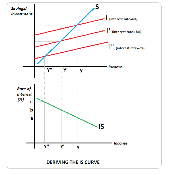
IS curve shows the various combinations of income and interest rate where savings is equal to investment. In the diagram below, in the upper panel we can see the savings and investment curves.

Copyright © 2021 Kalkine Media

Savings are positively related to income and thus is an upward sloping curve. Investment, on the other hand, depends on income and interest rate. At a given level of interest rate, say b%, investments keep increasing with the increase in income- this can be seen from the curve I'. If the interest rate increased to c%, lesser investments would correspond to each income level. This is so that the marginal efficiency of capital be raised to sync with the increased interest rate. If the interest rate falls to a%, then the investment curve will shift upwards to I". Again, the investments will have to be raised so that the marginal efficiency of capital falls to be in sync with the lower interest rate.

In the bottom panel of the graph, we see that the IS curve is derived by joining together the points which have savings-investment equality at various interest rates- income combinations. Thus, the IS curve is a downward sloping curve because as the interest rate decreases, there is an increase in investment and in income.

The IS curve can be said to be the goods market equilibrium derived as the inverse relationship between the economy's rate of interest and income.

What determines the slope of the IS curve?

The size of the multiplier has an impact on the slope of the IS curve. A higher multiplier value implies a higher income elasticity in response to a change in interest rate- this implies a flatter IS curve. An IS curve is more elastic when the percentage change in income is greater than the percentage change in the interest rate.

What causes shifts in the IS curve?

A rightward shift in the IS curve may be caused by increased consumption, investment, government expenditure, and net exports. A rightward shift may also be caused by a reduction in tax in the economy. Similarly, any adverse shocks to these variables will shift the IS curve to the left.

It may be noted that a change in interest rates will not shift the IS curve but will cause movements along the curve.

How do we arrive at the money market equilibrium?

The money market is in equilibrium when money demand (shown by L) in the economy is equal to the money supply (shown by M). Thus money market is said to be in equilibrium when L=M

L=Lt + Ls

Where

• Lt= transaction demand for money, which has a direct relationship with income. It is may be denoted as

• Lt= f(Y)

• Ls= speculative demand for money, which has a negative relationship with the rate of interest and is denoted as

• Ls=f(r)

How can the LM curve be derived?

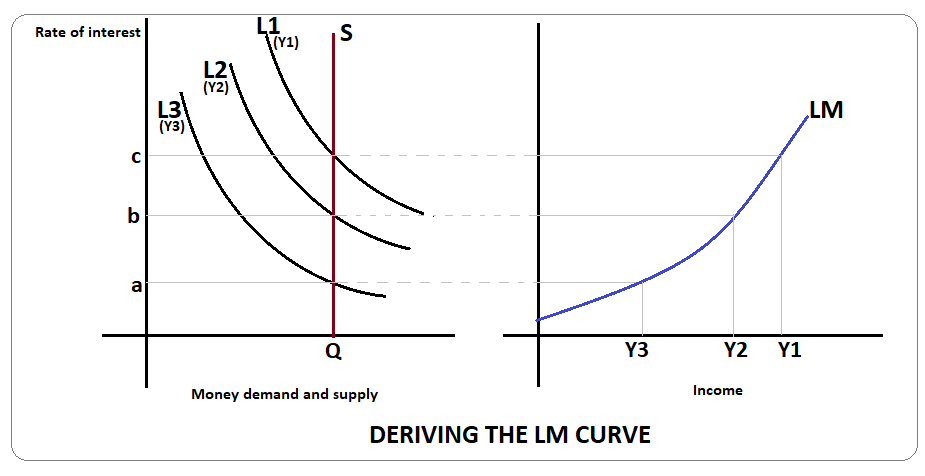
LM curve is the combination interest rates and income levels where money demand and money supply are equal. This is also called money market equilibrium.

In the diagram below, L1, L2, and L3 are liquidity preferences or money demand curves at income levels Y1, Y2, and Y3, respectively. Y1 > Y2 > Y3. The horizontal line QS is a vertical line indicating a constant or perfectly inelastic money supply in the economy. On the right panel is the LM curve, which shows the combination of interest rates and income where money demand equals money supply in the economy.

Copyright © 2021 Kalkine Media

What is the slope of the supply curve?

The LM curve is upward sloping from left to right. As income increases, there is an increase in demand for money in the economy, which leads to an increase in interest rates. Risen interest rates lead to a decline in demand for money, thus making it equal to the money supply. The lesser the income elasticity of money demand, the higher the interest rate elasticity of money demand and flatter will the LM curve be. A flatter LM curve implies that the interest rate elasticity of income is inelastic.

What causes shifts in the LM curve?

LM function is derived based on money demand and supply. Therefore, holding any one of these factors constant, an increase or decrease in the other variable will lead to a shift in the LM curve.

In the case of expansionary monetary policy, there is an increase in the money supply in the economy, shifting the LM curve to the right. Similarly, a decrease in money demand also creates excess money supply in the economy and thus shifts the LM curve to the right. On the other hand, an increase in money demand or a decrease in money supply will shift the LM curve to the left.

It may be noted that other things remaining constant, a change in the rate of interest will not shift the curve but only lead to a movement along the LM curve.

What is the IS-LM model?

Copyright © 2021 Kalkine Media

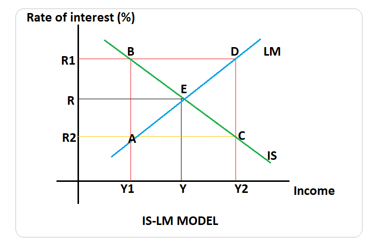
The IS-LM model is used to determine the income-interest rate combination wherein the goods market and the money market are in equilibrium. This equilibrium is attained at point E corresponding to interest R and income level Y in the above diagram. Thus, any deviation from E will trigger the market forces to revert to E.

Suppose we see income level Y1, the goods market is at equilibrium at R1 while the money market is in equilibrium at R2. At point A, investment is more than savings- implying an excess demand for goods. As a result, income increases. With higher income, there is more demand for transactions which is met by selling off bonds. This results in interest rates rising- inducing a movement along the LM curve from point A to E. Here the interest rate is higher, and thus investments are lower. At the same time, a higher income level leads to an increase in savings.

On the other hand, if the economy is at point C, where the interest rate is at level R2 and income is at level Y2. Here the goods market is in equilibrium, but the money market is not. Money market equilibrium can be attained at the Y2 level of income only when the interest rate is higher at R1, i.e. at point D. At C, the money demand exceeds the money supply at the lower interest rate R2. Due to the excess demand for money, bonds are sold off, and interest rates rise. An increase in interest rates leads to an upward movement along the IS curve from point C to E. On the LM curve, decreased income reduces transaction demand for money, and ultimately equilibrium is attained at E.